library(sf)
library(mapview)
library(adehabitatHR)
library(sp)
library(dplyr)
library(ggplot2)

# read in sf object
bou <- read_sf("clean_data/caribou.gpkg")

# add seasons
bou <- bou |>
  mutate(season = case_when(
            month %in% c(4,5) ~ "spring",
            month %in% c(6,7,8) ~ "summer",
            month %in% c(9,10,11) ~ "fall",
            month %in% c(12,1,2,3) ~ "winter"))

# add coordinates
tdf <- st_coordinates(bou) |>
    cbind(bou) |>
    dplyr::select(location.long, location.lat, herd, animal.id, season) |>
st_drop_geometry()Generating Home Range Estimates
Overview
In this module we will create home range estimates using minimum convex polygons and kernel density estimates (kde) exploring a range of methods available.
1. Preparation
Lets begin by checking we have enough points to be confident in our home range estimate. The total number of raw fixes will vary depending between individuals by season and years. In this example we will use a minimum of 50 unique locations as recommended for home range calculations (Seaman 1999, Kernohan 2001).
Note: telemetry data is yet to be subset by a specific time interval and currently includes all raw fixes.
id_pts <- tdf |>
      group_by(animal.id)|>
      summarise(count = n())

season_pts <- tdf |>
      group_by(herd, season)|>
      summarise(count = n())
2. Minimum Convex Polygons
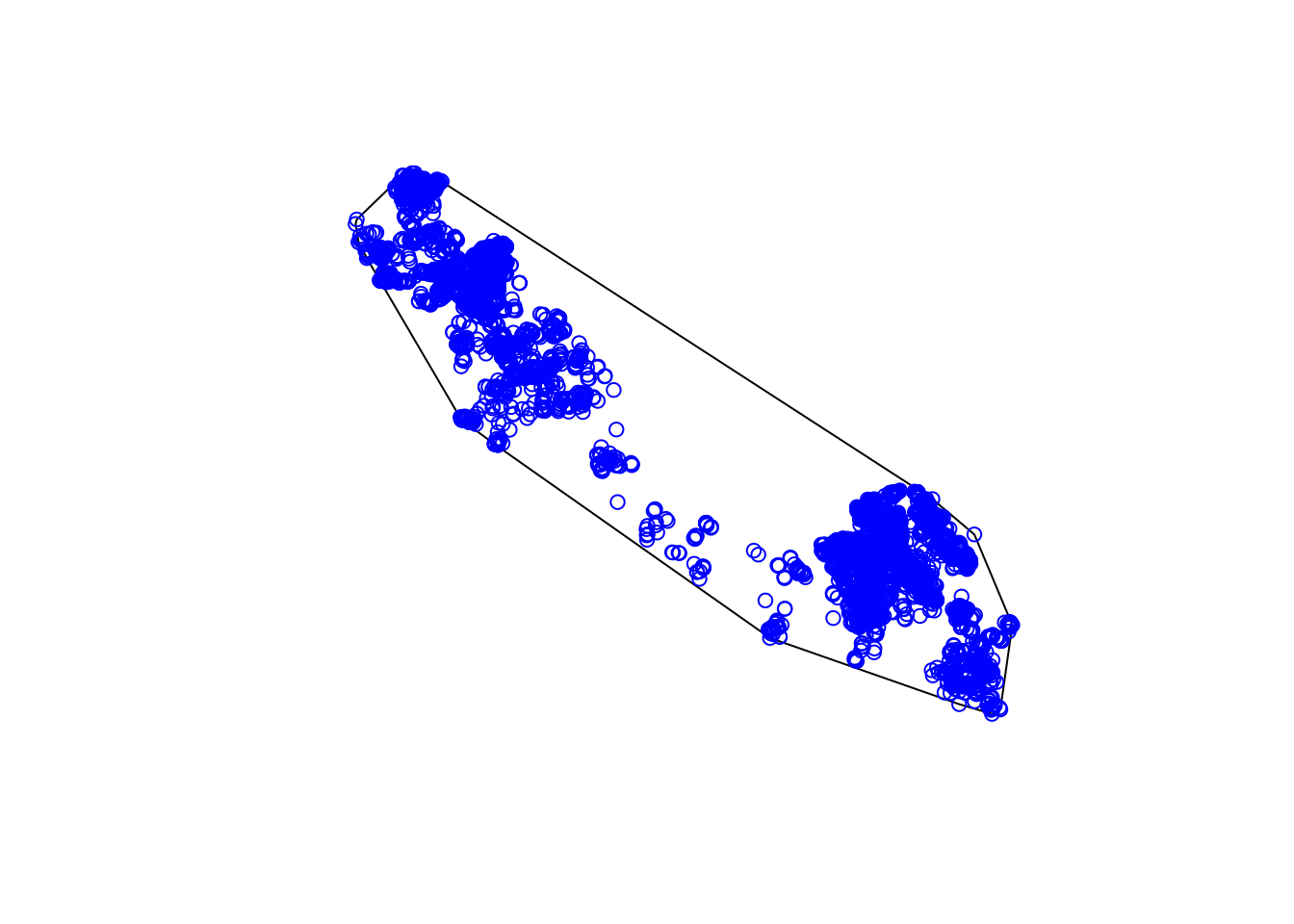
Minimum convex polygons (mcp) can be used to provide a quick estimate of data distribution. This provides a very broad brush approach and does not include density estimates.
2.1 Using the sf package.
This is not very representative so what other methods can we use?
2.2 Using the sp package.
Alternatively we can use the adhabitatHR package, which contains many ecology specific tools and functions. The downside of using this package is the reliance on old spatial package (sp) . The sp package has largely been superseded by the sf package. Unfortunately this is the reality of a coding language which is constantly being updated and improved!
The sp package uses a specific format called SpatialPointsDataFrame. To use these functions we need to convert from sf to sp formats.
#  Create SpatialPointsDataFrame object
  tdfgeo <- bou |>
    dplyr::select(animal.id) |>
    as("Spatial")

  # Calculate MCPs
  c.mcp <- mcp(tdfgeo, percent = 100)

  # convert this to a sf object
  c.mcp_sf <- st_as_sf(c.mcp)

  # plot with mapview
  mapview::mapview(c.mcp_sf)
The advantage of using the adhabitatHR package is that it provides many more outputs and enables us to customize the information we want. For example we can extract multiple home ranges based on varying levels of specificity; i.e. percent = 75%.
  # lets look at 75% inclusion
  c.mcp.75 <- mcp(tdfgeo, percent = 75)

   # Plot
  plot(tdfgeo, col = as.factor(tdfgeo$animal.id), pch = 16)
  plot(c.mcp , col = alpha(1:5, 0.5), add = TRUE)
  plot(c.mcp.75, col = alpha(1:5, 0.5), add = TRUE)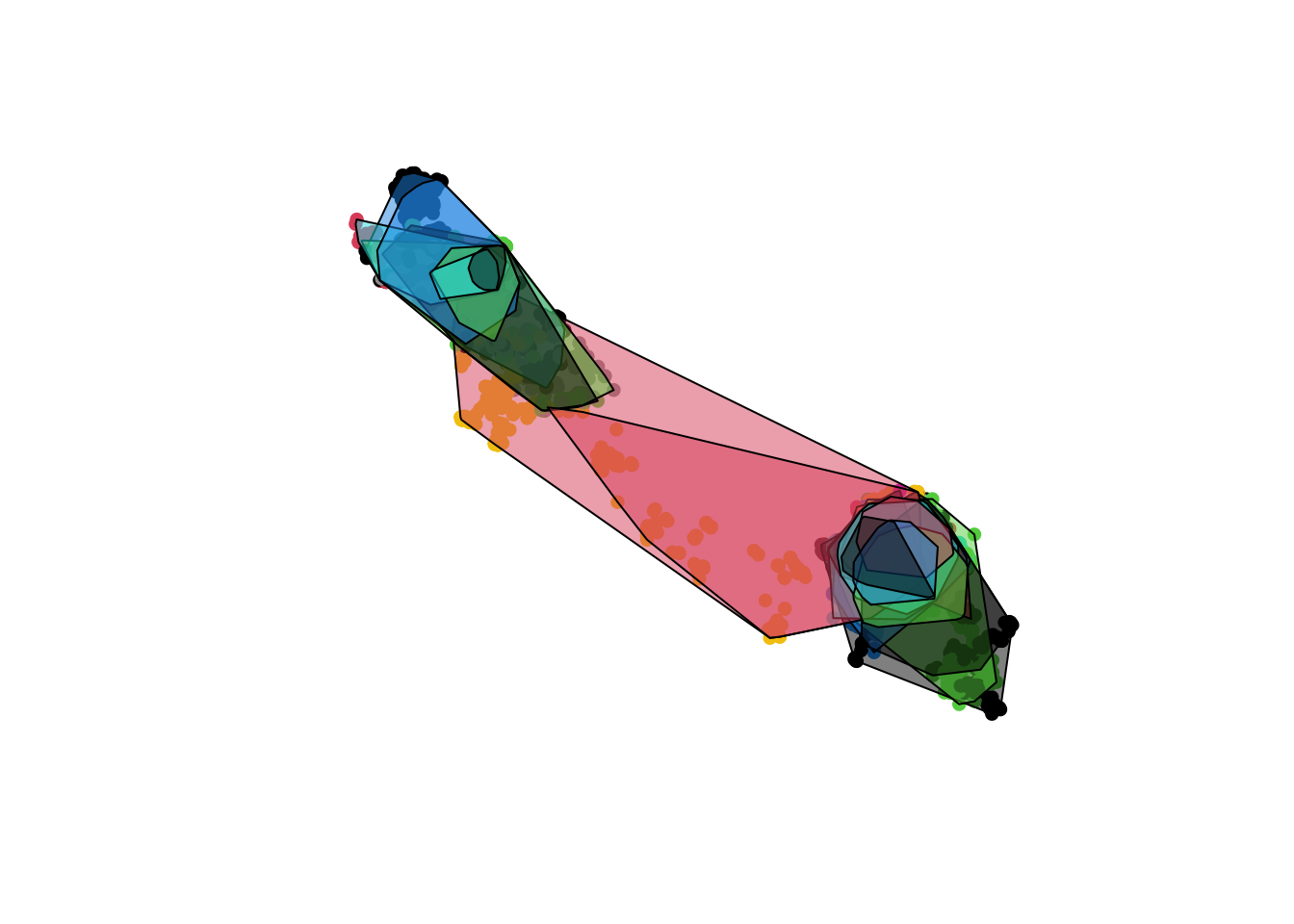
  # Calculate the MCP by including 50 to 100 percent of points
  hrarea <- mcp.area(tdfgeo, percent = seq(50, 100, by = 10))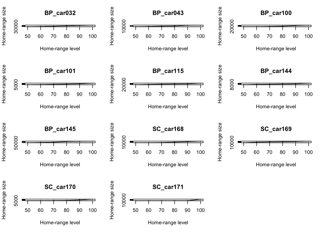
3. Kernel Density Estimates (kde)
Kernel Density Estimates (kde) are a popular method to estimate the distribution of data, hence are used to estimate home ranges. Calculations for KDE require consideration of the mathematical method to describe the density function. A detailed description of the parameters can be found here.
KDEs are very sensitive to input parameters, specifically the bandwidth (h) which determines the smoothing parameter. H parameters can be estimated using three methods:
- a reference bandwidth (h = σ × n ^−1/6), however this is generally an overestimate of the range, and is not suitable for multi-modal distributions.
- Least Square Cross Validation (LSCV), which minimizes the difference in volume between the true UD and the estimates UD.
- A subjective visual choice for the smoothing parameter, based on successive trials (Silverman, 1986; Wand & Jones 1995).
Other parameters include:
Kernel Type: The type of kernel is limited to Gaussian (bivariate normal), quadratic or normal. We used the bivariate normal model as default.
Grid/extent: These determines the area or extent over which the home range will be estimated. This is a mix of fine scale and time consuming processing and faster blocky resolution over a continuous surface. As a rule of thumb, Geospatial Modelling Environment program (GME) formally Hawth’s tools suggest: take the square root of the x or y variance value (whichever is smaller) and divide by 5 or 10 (I usually round to the nearest big number - so 36.7 becomes 40). Before using this rule of thumb value calculate how many cells this will result in for the output (take the width and height of you input points, divide by the cell size, and multiply the resulting numbers together). If you get a value somewhere between 1-20 million, then you have a reasonable value.
To create home ranges for each unique id we used a bivariate normal kernel with a variety of h (smoothing parameters). We then interpreted visually to determine size to use based on successive trials. This is supported by the literature (Hemson et al. 2005; Calenge et al. 2011).
It is also possible to run KDE with set barriers and boundaries.
3.1 kde: h reference parameter
tdfgeo <- bou |>
  dplyr::select(animal.id) |>
  as("Spatial")

# define the parameters (h, kern, grid, extent)
kde_href  <- kernelUD(tdfgeo, h = "href", kern = c("bivnorm"), grid = 500, extent = 2)

kde_href
********** Utilization distribution of several Animals ************
Type: probability density
Smoothing parameter estimated with a href smoothing parameter
This object is a list with one component per animal.
Each component is an object of class estUD
See estUD-class for more informationFrom this object (Utilization distribution of several Animals) we can extract the vertices or polygons which define the percentage we wish to include.
ver95 <- getverticeshr(kde_href,95) # get vertices for home range
ver95_sf <- st_as_sf(ver95)         # convert to sf object

ver75 <- getverticeshr(kde_href,75)
ver75_sf <- st_as_sf(ver75 )

ver50 <- getverticeshr(kde_href,50)
ver50_sf<- st_as_sf(ver50)

# plot the outputs
mapview(ver50_sf, zcol = "id")
mapview (ver75_sf, zcol = "id") mapview (ver95_sf, zcol = "id")plot(st_geometry(ver95_sf),col = "yellow")
plot(st_geometry(ver75_sf),col = "blue", add = TRUE)
plot(st_geometry(ver50_sf),col = "purple", add = TRUE)
plot(tdfgeo, pch = 1, size = 0.5, add = TRUE) # Add points 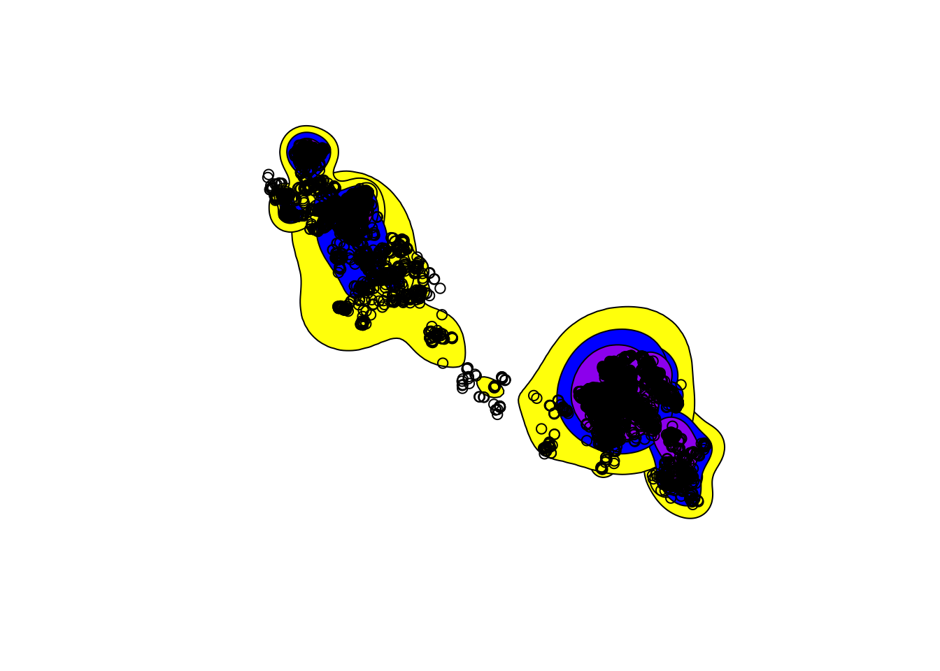
3.2 kde: Least Squares Cross Validation (lscv) method.
kde_lscv  <- kernelUD(tdfgeo, h = "LSCV", kern = c("bivnorm"), grid = 500, extent = 2)

ver95ls <- getverticeshr(kde_lscv,95) # get vertices for home range
ver95ls_sf <- st_as_sf(ver95ls)

ver50ls <- getverticeshr(kde_lscv,50)
ver50ls_sf <- st_as_sf(ver50ls)

# plot the outputs
mapview(ver50ls_sf, zcol = "id")
mapview (ver95ls_sf, zcol = "id")3.3 kde: variable smoothing parameters (h)
To test the sensitivity of the h value we can test a bivariate normal kernel with a variety of smoothing parameters (h = 1000, 2000, 4000).
We can then interpreted visually to determine size to use based on successive trials. This approach is supported by literature (Hemson et al. 2005; Calenge et al. 2011).
Lets extract the vertices and compare the outputs by building a plot.
# kde - href = 1000
ver95_1000 <- getverticeshr(kde_h1000, 95) # get vertices for home range
ver95_1000_sf <- st_as_sf(ver95_1000) |>     mutate(h = 1000) # convert to sf object

# kde - href = 500
ver95_500 <- getverticeshr(kde_h500, 95) # get vertices for home range
ver95_500_sf <- st_as_sf(ver95_500)  |>
  mutate(h = 500) # convert to sf object

# kde - href = 3000
ver95_3000 <- getverticeshr(kde_h3000, 95) # get vertices for home range
ver95_3000_sf <- st_as_sf(ver95_3000)  |>
  mutate(h = 3000) # convert to sf object

# bind all data together
all_verts <- bind_rows(ver95_1000_sf,  ver95_500_sf,  ver95_3000_sf)

# lets plot the output
ggplot(data = all_verts) +
geom_sf(
    aes(colour = id),
    alpha = 0.1
  ) +
  scale_colour_viridis_d() +
  facet_wrap(vars(h)) +
  theme_bw()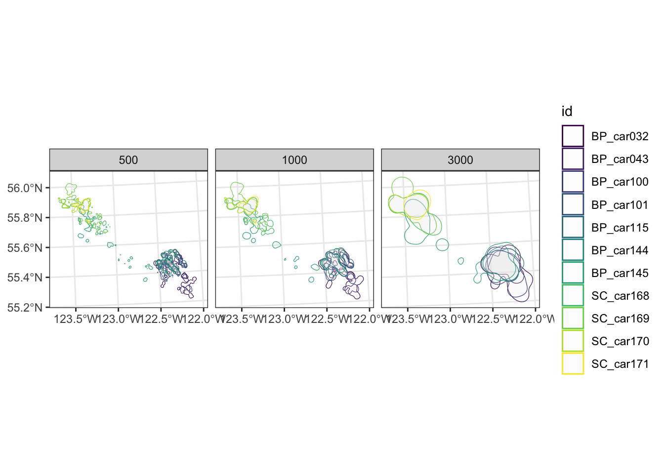
Comparison of kde parameters
Lets rerun the home range by season and compare the methods for the KDE.
tdfseason <- bou |>
  dplyr::filter(herd == "Burnt Pine") |>
  dplyr::select(season) |>
  as("Spatial")

# href
kde_href  <- kernelUD(tdfseason, h = "href", kern = c("bivnorm"), grid = 500, extent = 2)

# custome h values
kde_h1000  <- kernelUD(tdfseason, h = 1000, kern = c("bivnorm"), grid = 500,extent = 2)

# lscv
kde_lscv  <- kernelUD(tdfseason, h = "LSCV", kern = c("bivnorm"), grid = 500, extent = 2)


# build function to get vertices

get_verts <- function(in_kde, percent = 95, fieldname){

  ver <- getverticeshr(in_kde, percent) # get vertices for home range
  ver_sf <- st_as_sf(ver)  |>
    mutate(type = fieldname)

  return(ver_sf)
}


# genertate vertices for each KDE

href <- get_verts(kde_href, percent = 95, fieldname = "href")
h1000 <- get_verts(kde_h1000, percent = 95, fieldname = "h1000")
kde_lscv <- get_verts(kde_lscv, percent = 95, fieldname = "lscv")

# bind all data together
all_seasons <- bind_rows(href, h1000, kde_lscv)

# lets plot the output
ggplot(data = all_seasons) +
geom_sf(
    aes(colour = id),
    alpha = 0.1
  ) +
  scale_colour_viridis_d() +
  coord_sf() +
  facet_wrap(vars(type)) +
  theme_bw()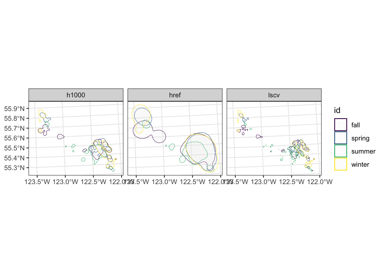
From this example we can see the large difference in home range estimates, depending on the type of method used and parameters selected.
When generating home range estimates it is important to think about the application of use, and test various parameters to estimate the best fit.
References
- Packages: Estimate Kernel home range Utilization Distribution Using adehabitatHR (Calenge et al. 2011)
- KDE
- https://www.ckwri.tamuk.edu/sites/default/files/publication/pdfs/2017/leonard_analyzing_wildlife_telemetry_data_in_r.pdf
- Seaman, D. E., Millspaugh, J. J., Kernohan, B. J., Brundige, G. C., Raedeke, K. J., & Gitzen, R. A. (1999). Effects of sample #size on kernel home range estimates. The journal of wildlife management, 739-747.
- Kernohan, B. J., R. A. Gitzen, and J. J. Millspaugh. 2001. Analysis of animal space use and movements. Pages 125–166 in J. J. #Millspaugh and J. M. Marzluff, editors. Radio tracking and animal populations. Academic Press, San Diego, CA, USA
- Hemson, G., Johnson, P., South, A., Kenward, R., Ripley, R., & MACDONALD, D. (2005). Are kernels the mustard? Data from global positioning system (GPS) collars suggests problems for kernel home‐range analyses with least‐squares cross‐validation. Journal of Animal Ecology, 74(3), 455-463
