Processing Base Vector Data

Overview:

In this module we will post-process vector data we prepared earlier using the terra package. This includes;

generate a road impact raster
calculate a distance to water raster
convert vectors to rasters
combine all rasters into a raster stack and export

1. Road influence

To assemble meaningful information for modelling, we often need to post-process vector data. This could include manipulating the data into categories (i.e. high, medium, low) or exploring spatial patterns in more detail (i.e. distance from a road)

In this example we will generate a raster to quantifying the impact of road type and spatial orientation.

# load in the libraries needed
library(bcdata)
library(sf)
library(dplyr)
library(terra)

# read in raster template
template <- rast("clean_data/template.tif")

# read in roads
roads <- read_sf("clean_data/roads.gpkg")

We can assume the impact of road type (ROAD_SURFACE) might have a different impact on Caribou avoidance or predator use.

We can use this column to assign values to reflect this. In this example we assign a higher value to roads that are likely to be traveled at a higher speed and would have more frequent use.

# assign a value to the roads based on estimated speed of travel or use
roads <- roads |>
  mutate(rd_value = case_when(
            ROAD_SURFACE == "loose" ~ 25,
            ROAD_SURFACE == "overgrown" ~ 5,
            ROAD_SURFACE == "rough" ~ 10,
            ROAD_SURFACE == "unknown" ~ 7.5))

Now we can convert the vector to a raster using the template

# convert roads to a raster 
rroads <- rasterize(roads, template, field = "rd_value" )

plot(rroads)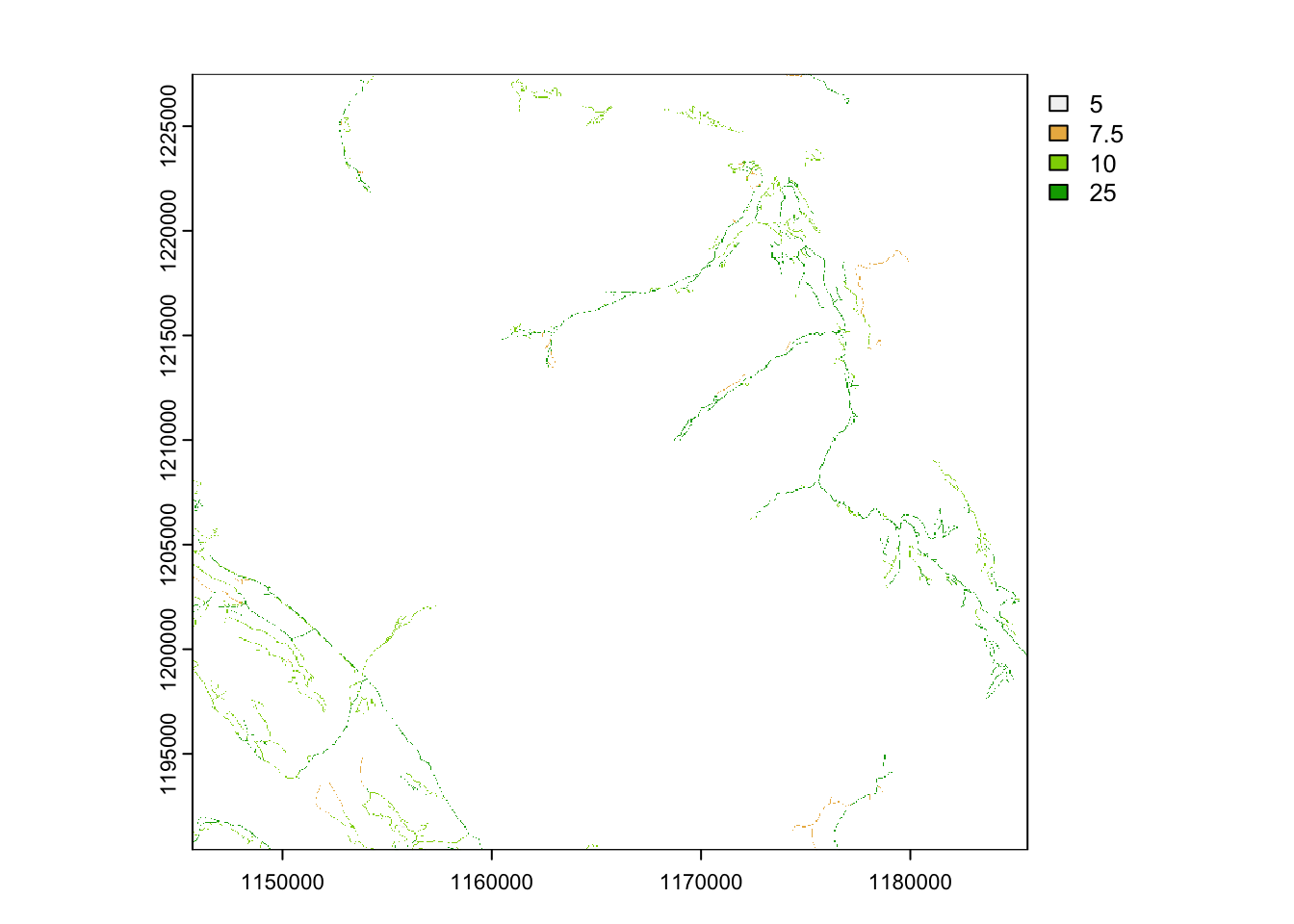

Secondly, we can assume the impact of the road will have a wider influence than a single pixel. To capture this influence we use a moving window analysis.

Moving windows or focal calculations estimate a new value for each pixel based on the values of the surrounding pixels (neighbours) and the function we supply. In this example we will use a window of 9, and a calculation based on the sum of these 9 pixels.

# create a moving window 
rrdens <- focal(rroads, w=9, fun="sum", na.rm=TRUE)

plot(rrdens)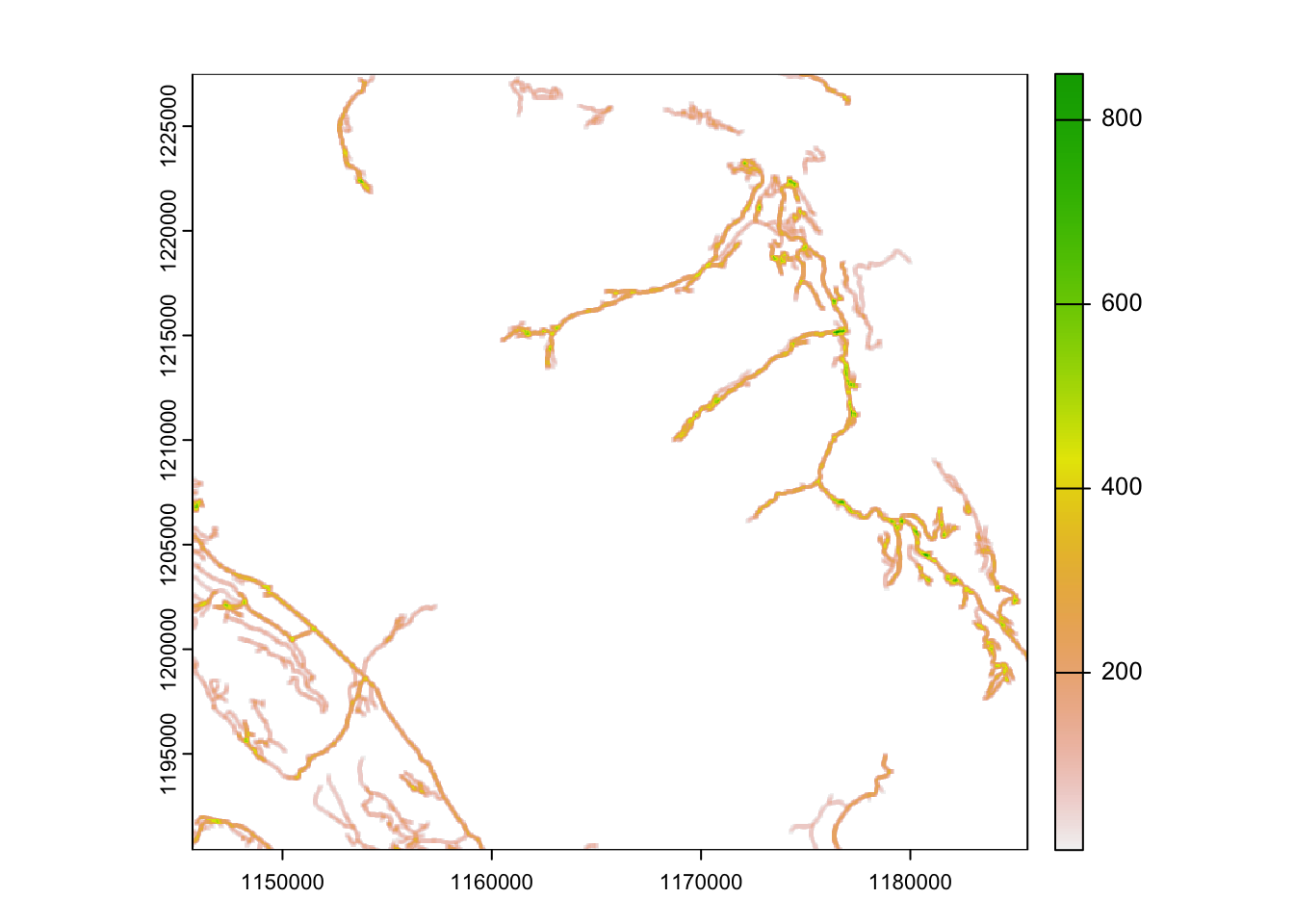

writeRaster(rrdens, "clean_data/road_density.tif", overwrite = TRUE)

2. Calculate distance from water

We might also be interested in understanding the relationship between Caribou locations and distance to a particular feature or habitat type.

In this case we will explore the distance to water bodies within the study areas.

# read in water 
water <- read_sf("clean_data/water.gpkg")

# calculate the distance to water for each pixel in the raster
# be patient - this might take some time. 
water_dis <- distance(template, water, unit = "km")


|---------|---------|---------|---------|
=========================================

plot(water_dis)
plot(water$geom, add = T)

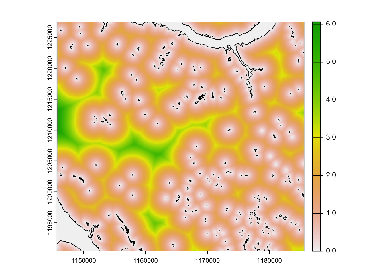
# what sort of values are we seeing?
range(water_dis)

class       : SpatRaster 
dimensions  : 1484, 1596, 2  (nrow, ncol, nlyr)
resolution  : 25, 25  (x, y)
extent      : 1145700, 1185600, 1190400, 1227500  (xmin, xmax, ymin, ymax)
coord. ref. : NAD83 / BC Albers (EPSG:3005) 
source(s)   : memory
names       : range_min, range_max 
min values  :  0.000000,  0.000000 
max values  :  6.090321,  6.090321

3. Convert base vector data to rasters

To prepare rasters for modelling and further analysis, we can convert all our vector data into one standard raster stack.

Note: it is not always required to convert to a raster stack, but this is helpful for any future predictions.

# read in our prepared vector data sets
bec <- read_sf("clean_data/bec.gpkg")
vri_conif <- read_sf("clean_data/vri_conif.gpkg")
vri_ageclass <- read_sf("clean_data/vri_ageclass.gpkg")
vri_cc <- read_sf("clean_data/vri_cc.gpkg")
cutblocks <- read_sf("clean_data/cutblocks.gpkg")
water <- read_sf("clean_data/water.gpkg")
streams <- read_sf("clean_data/streams.gpkg")
roads <- read_sf("clean_data/roads.gpkg")

# convert to rasters
rbec <- rasterize(bec, template, field = "MAP_LABEL")
rvri_conif <- rasterize(vri_conif, template, field = "conif")
rvri_ageclass <- rasterize(vri_ageclass, template, field = "age_class")
rvri_cc <- rasterize(vri_cc, template, field = "cc_class" )
rcutblocks <- rasterize(cutblocks, template, field = "HARVEST_YEAR")
rwater <- rasterize(water, template, field = "WATERBODY_TYPE" )
rstreams <- rasterize(streams, template, field = "STREAM_ORDER" )
rroads <- rasterize(roads, template, field = "ROAD_SURFACE" )

# stack into a set of rasters
vect_stack <- c(rbec, rvri_conif, rvri_ageclass, rvri_cc,
                rcutblocks, rwater, rstreams, rroads, 
                water_dis, rrdens)

plot(vect_stack)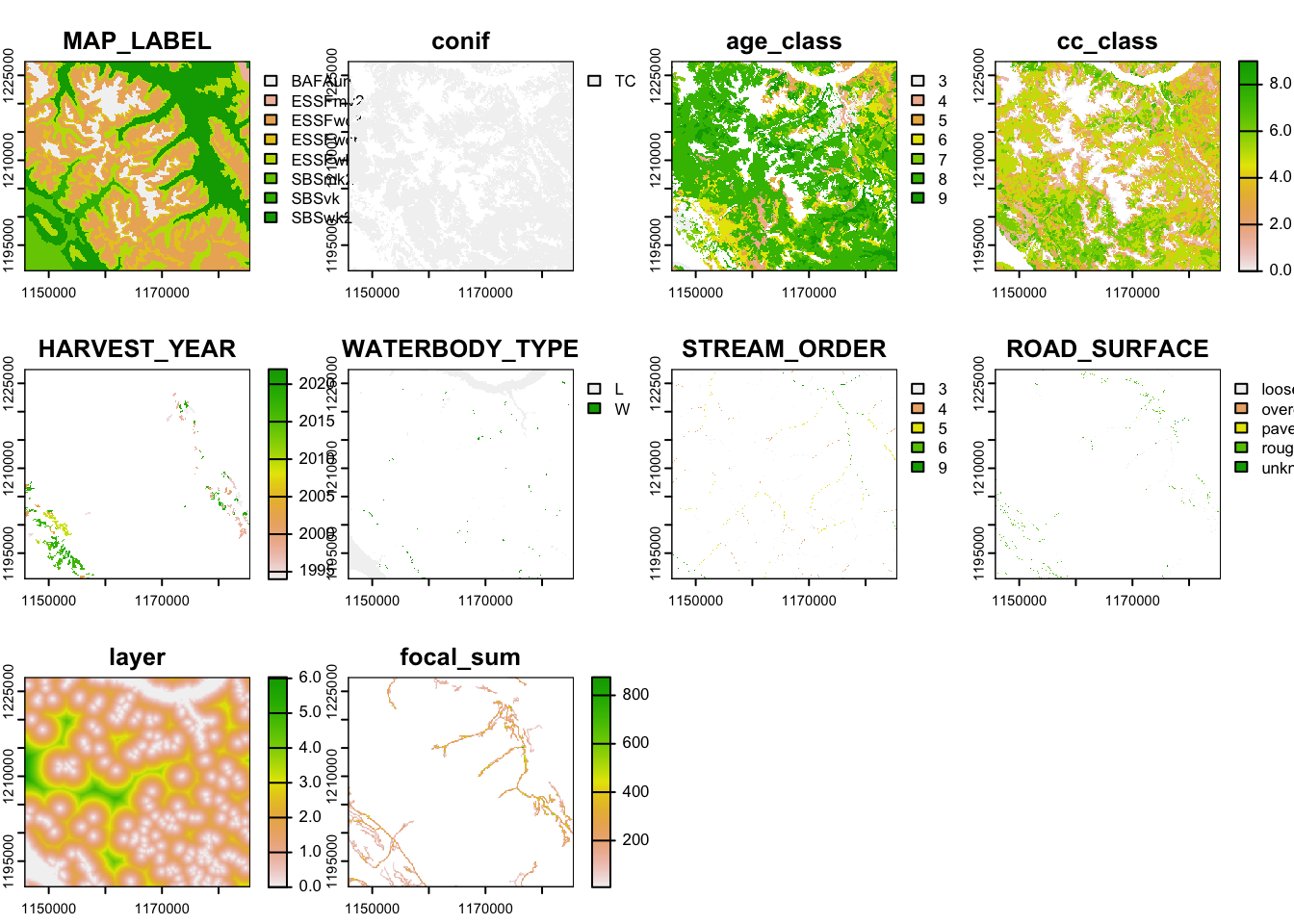

Lets combine these with the terrain rasters we created earlier.

rslope <- rast("clean_data/slope.tif")
raspect <- rast("clean_data/aspect.tif")
rtri  <- rast("clean_data/tri.tif")
rtrim_3005 <- rast("clean_data/dem.tif")

# create a raster stack
rast_stack <- c(rtrim_3005, rslope, raspect, rtri)

4. Combine raster layers into a stack

all_stack <- c(vect_stack, rast_stack)

plot(all_stack)

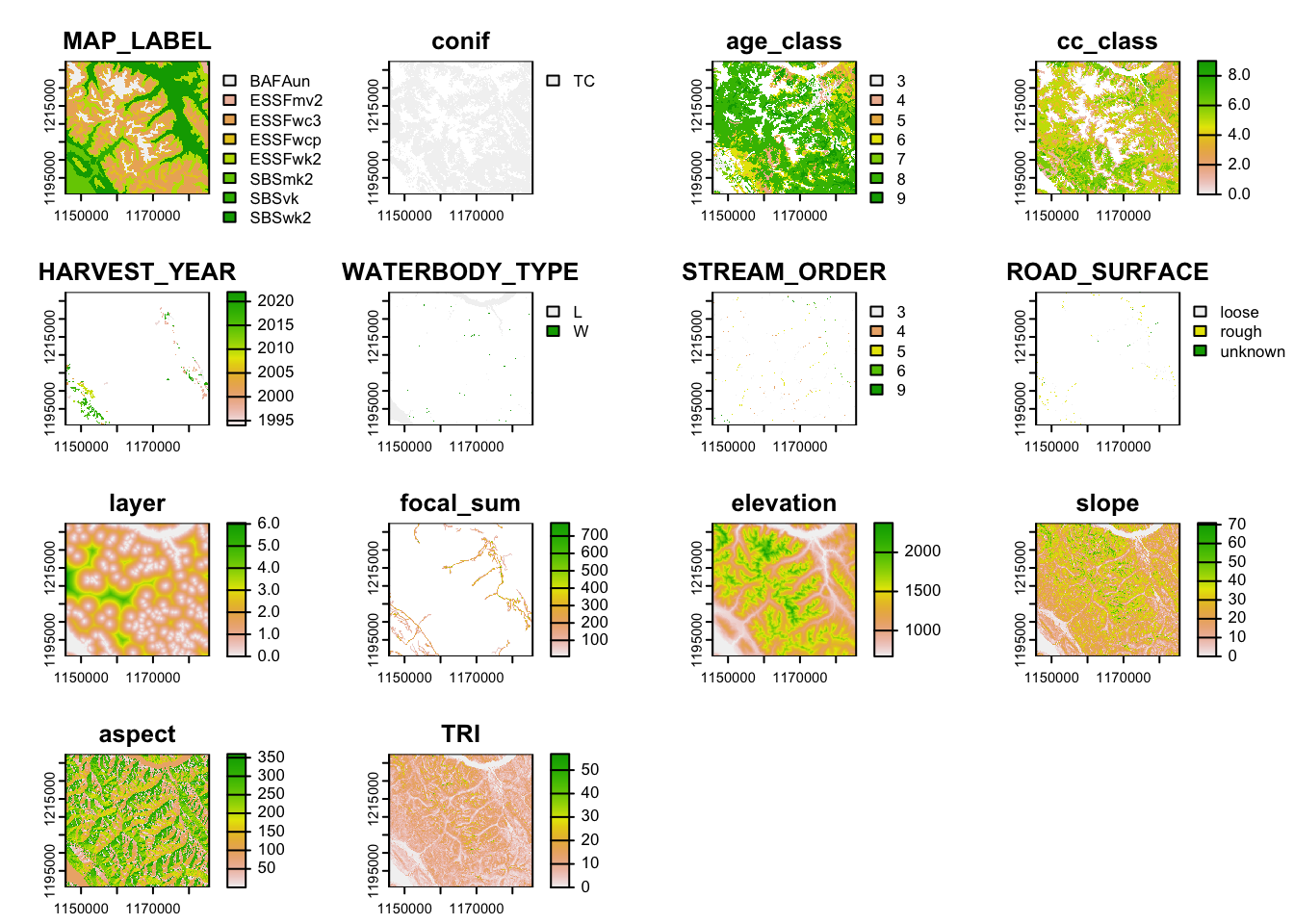
# we can write this out as a tif (raster object) 
#writeRaster(all_stack, "clean_data/rstack.tif", overwrite = T)

Or we can write this out to a very small R object

saveRDS(all_stack, "clean_data/covars.RDS") # much faster

Your turn

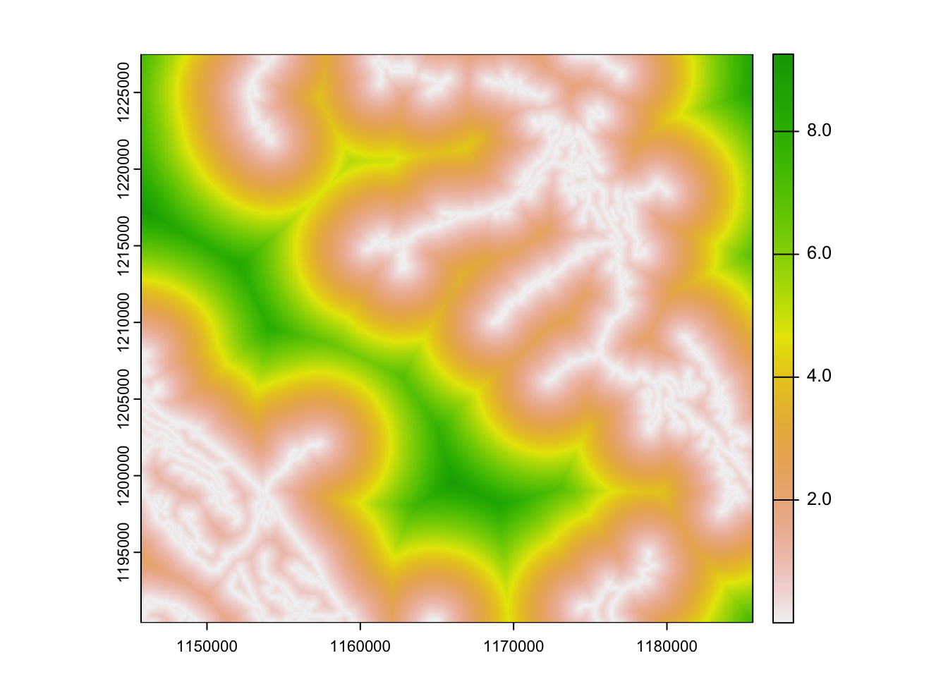
Generate a road density later using a different function (i.e. not sum), and or different scale of window (w). Hint: use the ?focal to see other options available.

Solution

# One example would be to generate the "max" value of the moving window. Note the w parameter is also reduced in the example. 
rrdensmax <- focal(rroads, w=3, fun="max", na.rm=TRUE)

Select another linear feature (roads, steams) and generate a raster to capture the distance to that feature for the study area.

Solution:

#This solution generates a distance from roads covariate
roads <- read_sf("clean_data/roads.gpkg") # read in roads

road_dis <- distance(template, roads, unit = "km") # calculate distance - be patient this might take time.


|---------|---------|---------|---------|
=========================================

plot(road_dis)