Generate random sample points for RSF

Overview:

In this module we use our prepared spatial data to generate the input data files to conduct a resource selection function analysis. This includes:

generate a set of “background points” from our study area.
extract spatial information for presence and background point locations
export as table for future use
generate summary statistics

Background: Resource Selection Functions

Now that we have a cleaned and standardized data set for the Scott Herd Caribou’s we can prepare the data for further analysis.

Resource Selection Functions are a common method used to assess what are the driving patterns of animal habitat preference. This process uses information or covariates (i.e. landscape attribute features) for locations where animals are present and compares them to all possible locations. In this way we can gather information on what conditions (i.e. landscape, aspect, distance from road, etc) characterize higher habitat use and selection for.

In addition to preparing data for future analysis, understanding the association with telemetry point locations and landscape information can provide meaningful summary statistics, i.e. proportion of locations within a specific BEC zone.

1. Generate background location points.

We will generate a simple set of “background points” based on the geographic distribution of the study area. Note you can limit the area in which these points are drawn from using more sophisticated methods, such as restricting points within a kernal density or home range estimate.

Lets start by reading in the libraries we will use.

library(dplyr)
library(terra)
library(sf)
library(mapview)
library(ggplot2)

Next, read in our point locations and rater template.

# read in the aoi template 
template <- rast("clean_data/template.tif")

# read in points 
bou_pts <- st_read("clean_data/scott_herd_subset.gpkg")

Reading layer `scott_herd_subset' from data source 
  `/Users/andy/dev/r-telemetry-workshop-nov-2023/clean_data/scott_herd_subset.gpkg' 
  using driver `GPKG'
Simple feature collection with 2906 features and 16 fields
Geometry type: POINT
Dimension:     XY
Bounding box:  xmin: 1145474 ymin: 1190327 xmax: 1185596 ymax: 1227451
Projected CRS: NAD83 / BC Albers

# Lets keep only the important columns and add a "presence/background" column. 
bou_pts <- bou_pts |>
  dplyr::select(animal.id, jdate)|>
  mutate(pres_bkg = 1)

We can use the spatSample function to generate random points for our given study area. This function has many more options which can be reviewed by using : ?spatSample in the console.

Lets generate a set of points the same length as our “presence” locations using a “random” method.

# Generate random points for RSF use areas.
set.seed(123)
avail_points <- spatSample(template, size = 2906, as.points = TRUE, na.rm = TRUE, method = "random")

avail_points <- st_as_sf(avail_points)

# lets rename the column to make it clear these are background points 
avail_points <- avail_points |>
  rename("pres_bkg" = aoi )

We can do a quick review of the points using mapview

mapview(avail_points) +
mapview(bou_pts, color = "red", cex= 3)

We can now combine our caribou locations and “background” locations into a single data set. We will retain the spatial information to allow us to easily extract the values in the corresponding raster stack

head(avail_points)

Simple feature collection with 6 features and 1 field
Geometry type: POINT
Dimension:     XY
Bounding box:  xmin: 1155662 ymin: 1195888 xmax: 1185438 ymax: 1225412
Projected CRS: NAD83 / BC Albers
  pres_bkg                geometry
1        0 POINT (1155662 1195888)
2        0 POINT (1185438 1225412)
3        0 POINT (1166262 1200912)
4        0 POINT (1179562 1198038)
5        0 POINT (1179038 1219712)
6        0 POINT (1162338 1221188)

head(bou_pts)

Simple feature collection with 6 features and 3 fields
Geometry type: POINT
Dimension:     XY
Bounding box:  xmin: 1164599 ymin: 1211860 xmax: 1165761 ymax: 1213029
Projected CRS: NAD83 / BC Albers
  animal.id jdate                    geom pres_bkg
1 SC_car168 15789 POINT (1164855 1211860)        1
2 SC_car168 15790 POINT (1164599 1211888)        1
3 SC_car168 15791 POINT (1165702 1212694)        1
4 SC_car168 15792 POINT (1165754 1212486)        1
5 SC_car168 15793 POINT (1165668 1213029)        1
6 SC_car168 15794 POINT (1165761 1212577)        1

allpts <- bind_rows(bou_pts, avail_points) 

head(allpts)

Simple feature collection with 6 features and 3 fields
Active geometry column: geom
Geometry type: POINT
Dimension:     XY
Bounding box:  xmin: 1164599 ymin: 1211860 xmax: 1165761 ymax: 1213029
Projected CRS: NAD83 / BC Albers
  animal.id jdate pres_bkg                    geom    geometry
1 SC_car168 15789        1 POINT (1164855 1211860) POINT EMPTY
2 SC_car168 15790        1 POINT (1164599 1211888) POINT EMPTY
3 SC_car168 15791        1 POINT (1165702 1212694) POINT EMPTY
4 SC_car168 15792        1 POINT (1165754 1212486) POINT EMPTY
5 SC_car168 15793        1 POINT (1165668 1213029) POINT EMPTY
6 SC_car168 15794        1 POINT (1165761 1212577) POINT EMPTY

# hmmmmm...........that looks weird what happened? 

# note we have slightly different column headers "geom" vs "geometry" 
st_geometry(avail_points) = "geom" 

allpts <- bind_rows(bou_pts, avail_points)

Extract point values

Next, we can read in our prepared raster stack as an .rds object. We can now use the extract function from the terra package to extract information for all layers in the raster stack for each of our points.

# read in the raster stack 
rstack <- readRDS("clean_data/covars.RDS")

# extract all values in the raster stack for each location in the bou_pts file. 
atts <- terra::extract(rstack, allpts)

head(atts)

  ID MAP_LABEL conif age_class cc_class HARVEST_YEAR WATERBODY_TYPE
1  1   ESSFwc3  <NA>        NA       NA           NA           <NA>
2  2   ESSFwc3    TC         9        5           NA           <NA>
3  3   ESSFwcp    TC         8        3           NA           <NA>
4  4   ESSFwcp    TC         8        3           NA           <NA>
5  5   ESSFwcp  <NA>         8        1           NA           <NA>
6  6   ESSFwcp    TC         8        3           NA           <NA>
  STREAM_ORDER ROAD_SURFACE     layer focal_sum elevation     slope     aspect
1           NA         <NA> 1.5773045        NA  1411.423 14.082280   2.045941
2           NA         <NA> 1.6258846        NA  1392.466 13.354155 320.360718
3           NA         <NA> 0.9053469        NA  1601.210  8.430601 138.105759
4           NA         <NA> 1.0990066        NA  1575.208  5.037906  95.403023
5           NA         <NA> 0.6147004        NA  1634.010  9.453105  94.128174
6           NA         <NA> 1.0157410        NA  1583.300  6.978374 175.275101
       TRI
1 4.809753
2 4.420059
3 2.718521
4 1.784927
5 3.197327
6 2.330856

# remove unused columns 
# Could show how to use st_write() and explain the cbind(st_coordinates()) bit
bou_full_pts <- cbind(allpts, atts) |>
  select(-ID)

Export as geo package or as csv table.

# spatial file 
write_sf(bou_full_pts, "clean_data/allpts_att.gpkg")

# write out as csv, keeping the XY values
bou_table <- st_coordinates(bou_full_pts) |> 
  cbind(bou_full_pts) |> 
  st_drop_geometry()

write.csv(bou_table, "clean_data/allpts_att.csv")

3. Summarise attributed point data

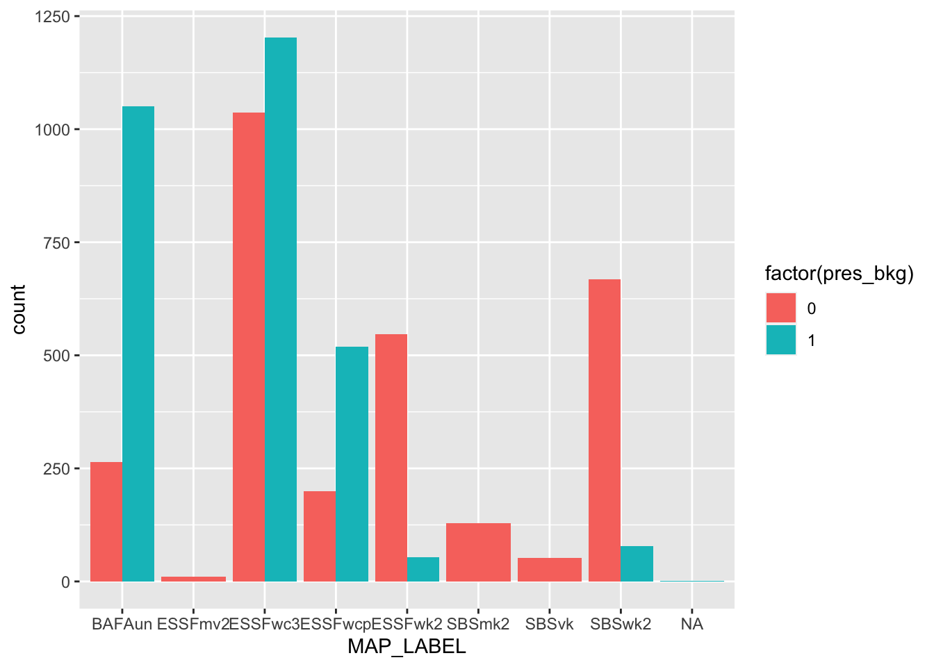
We can use our attributed point data to provide valuable summaries of landscape feature. Lets looks at aspect and BEC zones.

# Aspect
ggplot(bou_table, aes(aspect)) +
  geom_histogram(binwidth = 20) +
  facet_wrap(~pres_bkg)

Warning: Removed 8 rows containing non-finite values (`stat_bin()`).

# BEC zones 
ggplot(bou_table, aes(MAP_LABEL, group = pres_bkg, fill = factor(pres_bkg))) +
  geom_bar(position = "dodge", show.legend = TRUE)

Your turn

Generate a second set of background points used a method other than “random”.

Solution:

avail_pts_regular <- spatSample(template, size = 50, as.points = TRUE, na.rm = TRUE, method = "regular")
mapview(avail_pts_regular)

Use the bou_table we created above to explore other landscape patters. Build a ggplot to show the differences between the presence and background points.

Solution

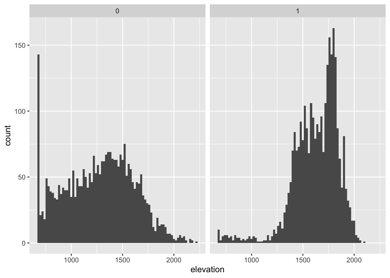
# Here are a few example using elevation and distance to water. 
# elevation 
ggplot(bou_table, aes(elevation)) +
  geom_histogram(binwidth = 20) +
  facet_wrap(~pres_bkg)

Warning: Removed 2 rows containing non-finite values (`stat_bin()`).

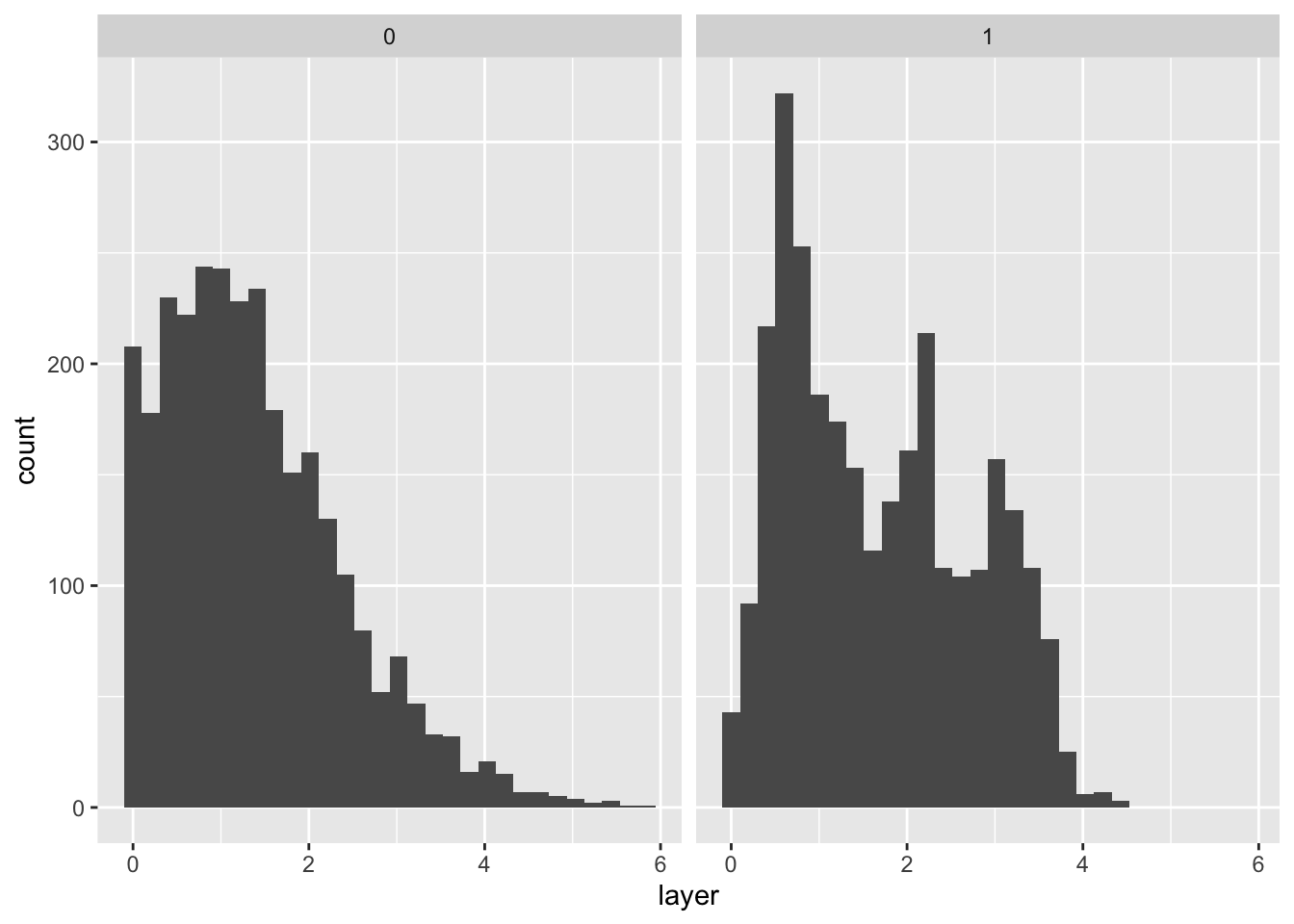
# distance to water (layer)
ggplot(bou_table, aes(layer)) +
  geom_histogram() +
  facet_wrap(~pres_bkg)

`stat_bin()` using `bins = 30`. Pick better value with `binwidth`.

Warning: Removed 2 rows containing non-finite values (`stat_bin()`).