Exploring Raster Data

Overview:

In this module we will explore raster data, and the available data sets which can be used in R for analysis. We will:

prepare our study aoi to use with rasters
extract DEM data through the bcmaps package
generate DEM derived covariates
prepare a raster stack with all spatial layers generated to date

Background: Rasters

Raster data is information built on a standard grid. These can be characterized by the grid extent (xmin, xmax, ymin, ymax) and can have a coordinate system to orient them in space. Rasters are made up of cells or pixels, based on a resolution or cell size. Each cell contains a single value. The terra package contains many functions for manipulating and processing rasters.

Note we will be using the BC Albers coordinate reference system (EPSG:3005). The advantages of this are 1) BCAlbers is an equal area projection across BC, 2) extent is marked using meters.

1. Create a standard raster template.

For ease of calculations we will create a standard “template” raster which will form the basis for all our data analysis.

# read in the libraries needed
library(dplyr)
library(sf)
library(bcmaps)
library(terra)

Read in our AOI that we made and saved previously. We can then convert this to a raster with a resolution of given size. In this example we will select 25m.

# read in the spatial file
bou <- read_sf("clean_data/scott_herd_subset.gpkg")

# read in the aoi previously created
aoi <- read_sf("clean_data/scott_aoi.gpkg")

We can now convert our polygon to a raster object.

# create a template raster with a resolution of 25m
template <- rast(aoi, resolution = 25, names = "aoi", vals = 0)

export the raster template for later processing

writeRaster(template, "clean_data/template.tif", overwrite = TRUE)

2. Extract base data using the CDED data set

Now we can use the bcmaps package to directly download digital elevation data from the Canadian Digital Elevation Model CDED. Within BC, this is largely equivalent to the TRIM DEM data set. We will use the cded_terra function.

# Note this is downloaded in tiles which will be cached 
trim_raw <- bcmaps::cded_terra(aoi)

checking your existing tiles for mapsheet 93o are up to date

checking your existing tiles for mapsheet 94b are up to date

trim_raw # note this is in WGS so we need to convert to 3005

class       : SpatRaster 
dimensions  : 1659, 3170, 1  (nrow, ncol, nlyr)
resolution  : 0.0002083333, 0.0002083333  (x, y)
extent      : -123.6772, -123.0168, 55.67445, 56.02008  (xmin, xmax, ymin, ymax)
coord. ref. : lon/lat NAD83 (EPSG:4269) 
source      : file15b9172c84853.vrt 
name        : elevation

res(trim_raw)

[1] 0.0002083333 0.0002083333

# reproject to match our raster template crs and extent
trim_3005 <- project(trim_raw, template)

# write out the individual raster
writeRaster(trim_3005, "clean_data/dem.tif", overwrite = TRUE)

3. Generate DEM derived covariates

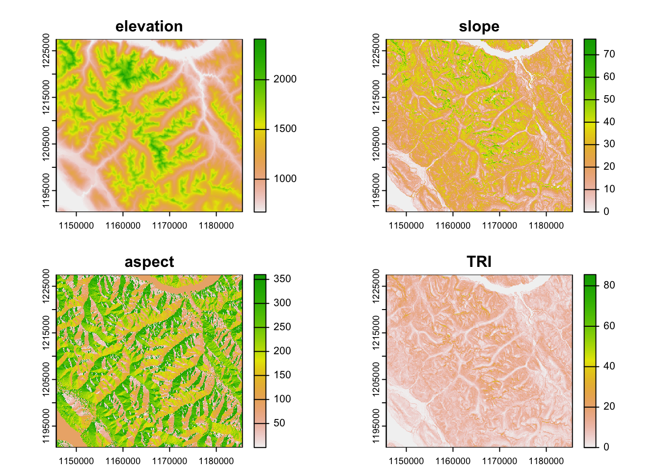
Now we can use the terrain functions within the terra package to generate some standard base layers derived from the DEM.

# generate slope 
rslope <- terrain(trim_3005, v = "slope", neighbors = 8, unit = "degrees") 

# generate aspect
aspect <- terrain(trim_3005, v = "aspect", neighbors = 8,  unit = "degrees") 

# generate topographic roughness index
tri <- terrain(trim_3005, v = "TRI", neighbors = 8)

# create a raster stack
rstack <- c(trim_3005, rslope, aspect, tri)

plot(rstack)

write our the individual rasters (.tif)

writeRaster(rslope, "clean_data/slope.tif", overwrite = TRUE)

writeRaster(aspect, "clean_data/aspect.tif", overwrite = TRUE)

writeRaster(tri, "clean_data/tri.tif", overwrite = TRUE)

Your Turn

Explore what other covariates you can generate using the terra::terrain function. Hint use ?terrain to see the help file.

Solution:

#There are a number of other options to select from including TPI, TRIriley, roughness, flowdir. 
#Use the ?terrain to find details on the parameters needed

?terra::terrain
roughness <-  terrain(trim_3005, v = "roughness") 
plot(roughness)

Compare outputs of aspect which the neighbours parameter is adjusted. What difference does this make to the output and the time to process?

Solution:

# generate aspect
aspect4 <- terrain(trim_3005, v = "aspect", neighbors = 4,  unit = "degrees") 

# generate aspect
aspect8 <- terrain(trim_3005, v = "aspect", neighbors = 8,  unit = "degrees") 

# use the window to check 
plot(aspect4)
plot(aspect8)

# Explore the change in metric if any
aspectrr <- terrain(trim_3005, v = "aspect", neighbors = 8,  unit = "radians")