Using R for Wildlife Telemetry Data Analysis - Introduction to Spatial Data with R

Outline

Introduction to Simple Features and the sf package
Coordinate Reference Systems
Reading various spatial data formats into R
Basic operations with spatial data

Learning objectives

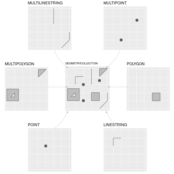
The “simple features” representation of vector data
Use and understand sf objects in R
Basic understanding of Coordinate Reference Systems (CRS)
Use mapview and sf to preview spatial data
How to do basic operations with spatial data using sf

Before we start

Configure RStudio
Get the course materials (if you haven’t already):

usethis::use_course(
  "https://github.com/ninoxconsulting/r-telemetry-workshop-nov-2023/raw/main/r-telemetry-workshop.zip"
)

<etherpad.andyteucher.ca/p/r-telemetry-pg>

Vector: Simple Features

The `sf` R package¹

Replaces

sp
rgdal
rgeos

Simple Features ²

Reading & previewing spatial data

library(sf)
library(mapview)

airports <- read_sf(
  "raw_data/bc_airports.gpkg"
)

mapview(airports)

mapview

mapview(airports, zcol = "NUMBER_OF_RUNWAYS")

Structure of an `sf` object

airports

Simple feature collection with 455 features and 5 fields
Geometry type: POINT
Dimension:     XY
Bounding box:  xmin: 406543.7 ymin: 367957.6 xmax: 1796645 ymax: 1689146
Projected CRS: NAD83 / BC Albers
# A tibble: 455 × 6
   AIRPORT_NAME                   IATA_CODE LOCALITY ELEVATION NUMBER_OF_RUNWAYS
   <chr>                          <chr>     <chr>        <dbl>             <int>
 1 Terrace (Northwest Regional) … <NA>      Terrace     217.                   2
 2 Victoria Harbour (Camel Point… <NA>      Victoria      4.57                 0
 3 Victoria Inner Harbour Airpor… YWH       Victoria      0                    0
 4 Victoria Harbour (Shoal Point… <NA>      Victoria      3.05                 0
 5 Victoria (Royal Jubilee Hospi… <NA>      Saanich      15.6                  0
 6 Victoria (General Hospital) H… <NA>      View Ro…     15.8                  0
 7 Victoria (BC Hydro) Heliport   <NA>      Saanich      12.2                  0
 8 San Juan Point (Coast Guard) … <NA>      Port Re…      7.62                 0
 9 Shawnigan Lake Water Aerodrome <NA>      Shawnig…      0                    0
10 Victoria International Airport YYJ       North S…     19.5                  3
# ℹ 445 more rows
# ℹ 1 more variable: geom <POINT [m]>

Key features of an `sf` object

st_geometry(airports)

Geometry set for 455 features 
Geometry type: POINT
Dimension:     XY
Bounding box:  xmin: 406543.7 ymin: 367957.6 xmax: 1796645 ymax: 1689146
Projected CRS: NAD83 / BC Albers
First 5 geometries:

POINT (833323.9 1054950)

POINT (1193727 381604.1)

POINT (1194902 382257.7)

POINT (1193719 382179.3)

POINT (1198292 383563.6)

st_bbox(airports)

     xmin      ymin      xmax      ymax 
 406543.7  367957.6 1796645.0 1689145.9

st_crs(airports)

Coordinate Reference System:
  User input: NAD83 / BC Albers 
  wkt:
PROJCRS["NAD83 / BC Albers",
    BASEGEOGCRS["NAD83",
        DATUM["North American Datum 1983",
            ELLIPSOID["GRS 1980",6378137,298.257222101,
                LENGTHUNIT["metre",1]]],
        PRIMEM["Greenwich",0,
            ANGLEUNIT["degree",0.0174532925199433]],
        ID["EPSG",4269]],
    CONVERSION["British Columbia Albers",
        METHOD["Albers Equal Area",
            ID["EPSG",9822]],
        PARAMETER["Latitude of false origin",45,
            ANGLEUNIT["degree",0.0174532925199433],
            ID["EPSG",8821]],
        PARAMETER["Longitude of false origin",-126,
            ANGLEUNIT["degree",0.0174532925199433],
            ID["EPSG",8822]],
        PARAMETER["Latitude of 1st standard parallel",50,
            ANGLEUNIT["degree",0.0174532925199433],
            ID["EPSG",8823]],
        PARAMETER["Latitude of 2nd standard parallel",58.5,
            ANGLEUNIT["degree",0.0174532925199433],
            ID["EPSG",8824]],
        PARAMETER["Easting at false origin",1000000,
            LENGTHUNIT["metre",1],
            ID["EPSG",8826]],
        PARAMETER["Northing at false origin",0,
            LENGTHUNIT["metre",1],
            ID["EPSG",8827]]],
    CS[Cartesian,2],
        AXIS["(E)",east,
            ORDER[1],
            LENGTHUNIT["metre",1]],
        AXIS["(N)",north,
            ORDER[2],
            LENGTHUNIT["metre",1]],
    USAGE[
        SCOPE["Province-wide spatial data management."],
        AREA["Canada - British Columbia."],
        BBOX[48.25,-139.04,60.01,-114.08]],
    ID["EPSG",3005]]

An `sf` object is a `data.frame`

class(airports)

[1] "sf"         "tbl_df"     "tbl"        "data.frame"

is.data.frame(airports)

[1] TRUE

summary(airports)

 AIRPORT_NAME        IATA_CODE           LOCALITY           ELEVATION     
 Length:455         Length:455         Length:455         Min.   :   0.0  
 Class :character   Class :character   Class :character   1st Qu.:   0.0  
 Mode  :character   Mode  :character   Mode  :character   Median :   6.4  
                                                          Mean   : 194.4  
                                                          3rd Qu.: 307.1  
                                                          Max.   :1277.4  
 NUMBER_OF_RUNWAYS            geom    
 Min.   :0.0000    POINT        :455  
 1st Qu.:0.0000    epsg:3005    :  0  
 Median :0.0000    +proj=aea ...:  0  
 Mean   :0.3385                       
 3rd Qu.:1.0000                       
 Max.   :3.0000

Coordinate Reference Systems

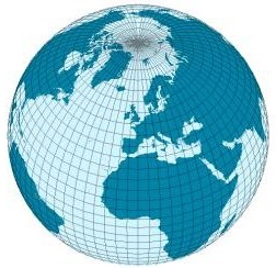
Geographic

spherical or ellipsoidal surface
ellipsoid defined by the datum
lat/long, measured in angular distances (degrees/radians)

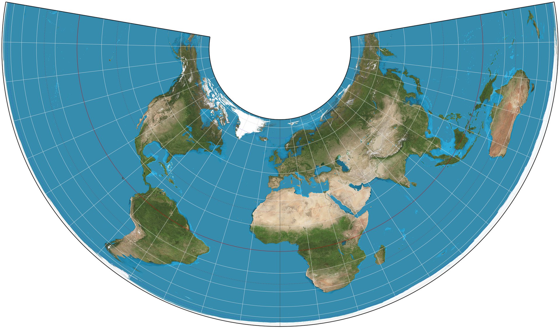
Projected

Cartesian coordinates on a flat plane
origin, x and y axes, linear unit of measurement (e.g., m)

defines how the spatial elements of the data relate to the surface of the Earth

Geographic: - identify any location on the Earth’s surface using two values — longitude and latitude. - Longitude is location in the East-West direction in angular distance from the Prime Meridian plane. - Latitude is angular distance North or South of the equatorial plane. - Distances in geographic CRSs are therefore not measured in meters. This has important consequences

Projected: - based on a geographic CRS - rely on map projections to convert the three-dimensional surface of the Earth into Easting and Northing (x and y) values in a projected CRS - often named based on a property they preserve: equal-area preserves area, azimuthal preserve direction, equidistant preserve distance, and conformal preserve local shape. - conic, cylindrical, planar

CRSs in R: EPSG codes

st_crs(airports)$input

[1] "NAD83 / BC Albers"

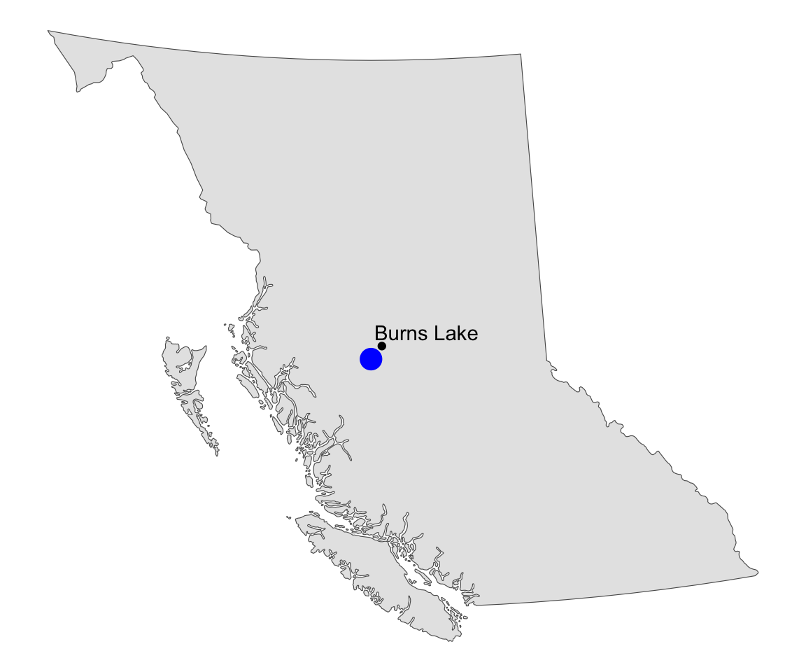
BC Albers - B.C.’s standard projection

Equal Area conic
Centre: c(-126, 54)

https://epsg.io/3005

WKT (Well-Known Text)

st_crs(3005)

Coordinate Reference System:
  User input: EPSG:3005 
  wkt:
PROJCRS["NAD83 / BC Albers",
    BASEGEOGCRS["NAD83",
        DATUM["North American Datum 1983",
            ELLIPSOID["GRS 1980",6378137,298.257222101,
                LENGTHUNIT["metre",1]]],
        PRIMEM["Greenwich",0,
            ANGLEUNIT["degree",0.0174532925199433]],
        ID["EPSG",4269]],
    CONVERSION["British Columbia Albers",
        METHOD["Albers Equal Area",
            ID["EPSG",9822]],
        PARAMETER["Latitude of false origin",45,
            ANGLEUNIT["degree",0.0174532925199433],
            ID["EPSG",8821]],
        PARAMETER["Longitude of false origin",-126,
            ANGLEUNIT["degree",0.0174532925199433],
            ID["EPSG",8822]],
        PARAMETER["Latitude of 1st standard parallel",50,
            ANGLEUNIT["degree",0.0174532925199433],
            ID["EPSG",8823]],
        PARAMETER["Latitude of 2nd standard parallel",58.5,
            ANGLEUNIT["degree",0.0174532925199433],
            ID["EPSG",8824]],
        PARAMETER["Easting at false origin",1000000,
            LENGTHUNIT["metre",1],
            ID["EPSG",8826]],
        PARAMETER["Northing at false origin",0,
            LENGTHUNIT["metre",1],
            ID["EPSG",8827]]],
    CS[Cartesian,2],
        AXIS["(E)",east,
            ORDER[1],
            LENGTHUNIT["metre",1]],
        AXIS["(N)",north,
            ORDER[2],
            LENGTHUNIT["metre",1]],
    USAGE[
        SCOPE["Province-wide spatial data management."],
        AREA["Canada - British Columbia."],
        BBOX[48.25,-139.04,60.01,-114.08]],
    ID["EPSG",3005]]

Your turn

Read in the electoral districts data in the `raw_data` folder:

What type of geometry is it?
What is the CRS?
What is the EPSG code?

Solution

elec_bc <- read_sf("raw_data/bc_electoral_districts.shp")
st_geometry_type(elec_bc, by_geometry = FALSE)

[1] POLYGON
18 Levels: GEOMETRY POINT LINESTRING POLYGON MULTIPOINT ... TRIANGLE

st_crs(elec_bc)

Coordinate Reference System:
  User input: WGS 84 
  wkt:
GEOGCRS["WGS 84",
    DATUM["World Geodetic System 1984",
        ELLIPSOID["WGS 84",6378137,298.257223563,
            LENGTHUNIT["metre",1]]],
    PRIMEM["Greenwich",0,
        ANGLEUNIT["degree",0.0174532925199433]],
    CS[ellipsoidal,2],
        AXIS["latitude",north,
            ORDER[1],
            ANGLEUNIT["degree",0.0174532925199433]],
        AXIS["longitude",east,
            ORDER[2],
            ANGLEUNIT["degree",0.0174532925199433]],
    ID["EPSG",4326]]

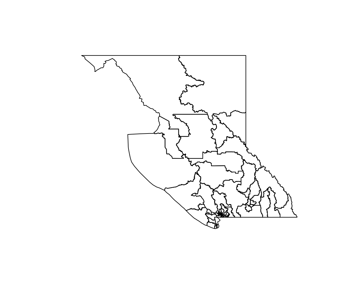
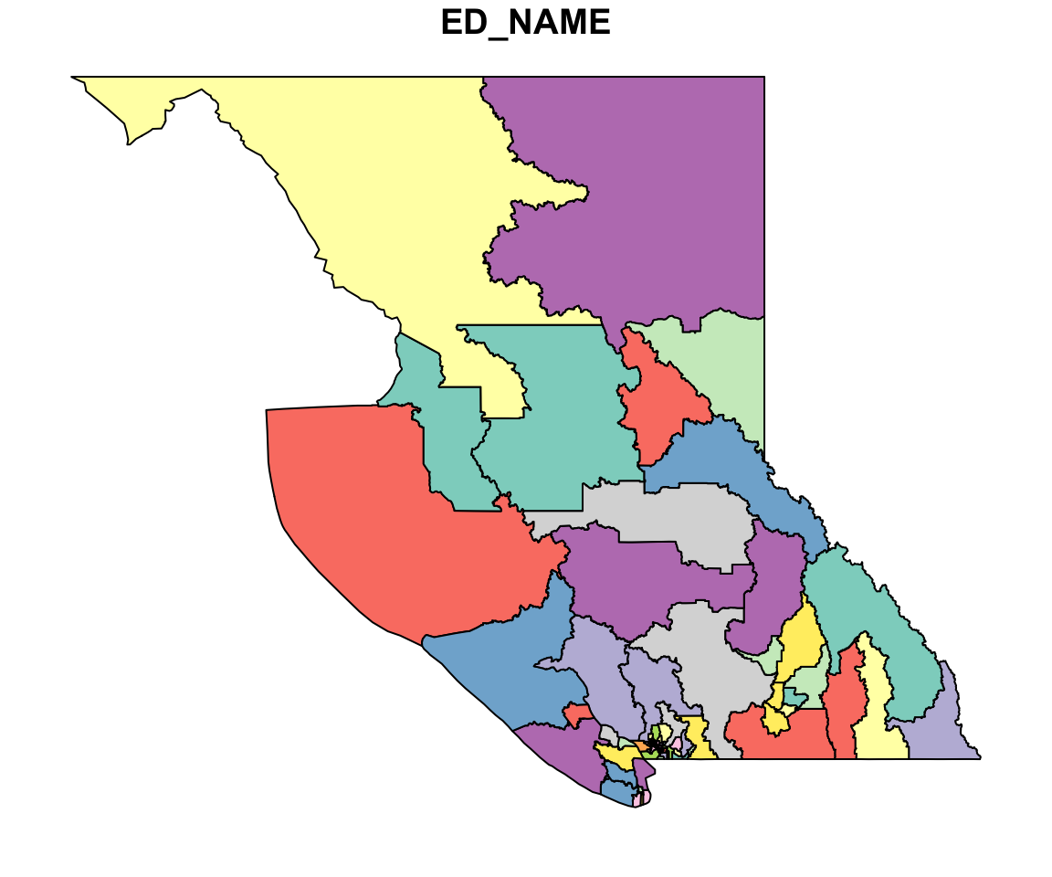
https://epsg.io/4326

Basic plotting

plot(elec_bc)

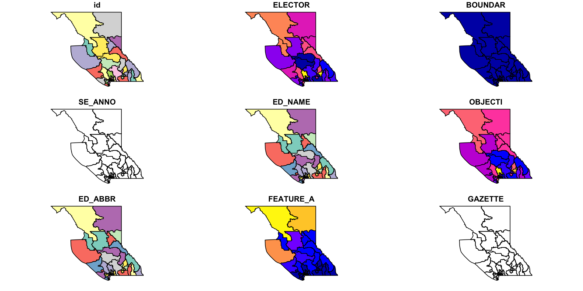
Basic plotting

Just the shapes

plot(st_geometry(elec_bc))

A single column

plot(elec_bc["ED_NAME"])

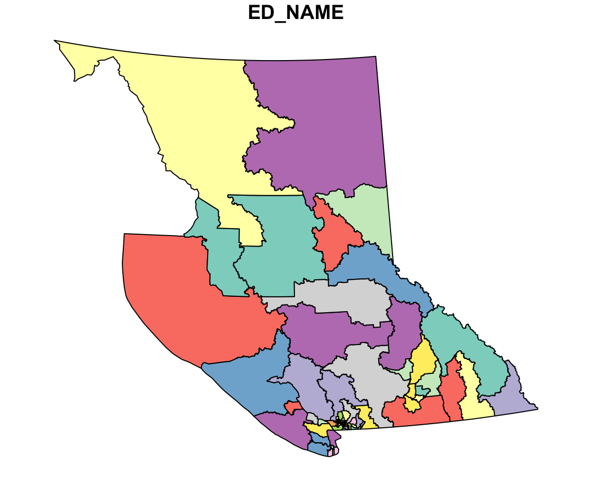
Transforming coordinate systems

elec_bc_albers <- st_transform(elec_bc, 3005)

Or, if you have another object in the CRS you want to use:

elec_bc_albers <- st_transform(elec_bc, st_crs(airports))
st_crs(elec_bc_albers)

Coordinate Reference System:
  User input: NAD83 / BC Albers 
  wkt:
PROJCRS["NAD83 / BC Albers",
    BASEGEOGCRS["NAD83",
        DATUM["North American Datum 1983",
            ELLIPSOID["GRS 1980",6378137,298.257222101,
                LENGTHUNIT["metre",1]]],
        PRIMEM["Greenwich",0,
            ANGLEUNIT["degree",0.0174532925199433]],
        ID["EPSG",4269]],
    CONVERSION["British Columbia Albers",
        METHOD["Albers Equal Area",
            ID["EPSG",9822]],
        PARAMETER["Latitude of false origin",45,
            ANGLEUNIT["degree",0.0174532925199433],
            ID["EPSG",8821]],
        PARAMETER["Longitude of false origin",-126,
            ANGLEUNIT["degree",0.0174532925199433],
            ID["EPSG",8822]],
        PARAMETER["Latitude of 1st standard parallel",50,
            ANGLEUNIT["degree",0.0174532925199433],
            ID["EPSG",8823]],
        PARAMETER["Latitude of 2nd standard parallel",58.5,
            ANGLEUNIT["degree",0.0174532925199433],
            ID["EPSG",8824]],
        PARAMETER["Easting at false origin",1000000,
            LENGTHUNIT["metre",1],
            ID["EPSG",8826]],
        PARAMETER["Northing at false origin",0,
            LENGTHUNIT["metre",1],
            ID["EPSG",8827]]],
    CS[Cartesian,2],
        AXIS["(E)",east,
            ORDER[1],
            LENGTHUNIT["metre",1]],
        AXIS["(N)",north,
            ORDER[2],
            LENGTHUNIT["metre",1]],
    USAGE[
        SCOPE["Province-wide spatial data management."],
        AREA["Canada - British Columbia."],
        BBOX[48.25,-139.04,60.01,-114.08]],
    ID["EPSG",3005]]

WGS 84 (EPSG: 4326)

plot(elec_bc[, "ED_NAME"])

BC Albers (EPSG: 3005)

plot(elec_bc_albers[, "ED_NAME"])

Your turn

Load "raw_data/ski_resorts.csv" as an sf object

facility_name	locality	latitude	longitude	elevation
Wapiti Ski Club	Elkford	50.02168	-114.9380	1467
Summit Lake Ski Area	Nakusp	50.14546	-117.6144	1132
Sasquatch Mountain Resort	Hemlock Valley	49.38011	-121.9354	1185
Apex Mountain Resort	Apex	49.39042	-119.9047	1852
Salmo Ski Hill	Salmo	49.18640	-117.3015	864
Red Mountain Resort	Rossland	49.10238	-117.8194	1150

Hints:

Load "raw_data/ski_resorts.csv" as an sf object

ski_resorts <- read.csv("raw_data/ski_resorts.csv")
ski_resorts <- st_as_sf(ski_resorts, ...)

Solution

ski_resorts <- read.csv("raw_data/ski_resorts.csv")

ski_resorts <- st_as_sf(ski_resorts,
                        coords = c("longitude", "latitude"),
                        crs = 4326)

head(ski_resorts)

Simple feature collection with 6 features and 3 fields
Geometry type: POINT
Dimension:     XY
Bounding box:  xmin: -121.9354 ymin: 49.10238 xmax: -114.938 ymax: 50.14546
Geodetic CRS:  WGS 84
              facility_name       locality elevation                   geometry
1           Wapiti Ski Club        Elkford      1467  POINT (-114.938 50.02168)
2      Summit Lake Ski Area         Nakusp      1132 POINT (-117.6144 50.14546)
3 Sasquatch Mountain Resort Hemlock Valley      1185 POINT (-121.9354 49.38011)
4      Apex Mountain Resort           Apex      1852 POINT (-119.9047 49.39042)
5            Salmo Ski Hill          Salmo       864  POINT (-117.3015 49.1864)
6       Red Mountain Resort       Rossland      1150 POINT (-117.8194 49.10238)

Geometric calculations

Geometric Measurements

st_area()
st_length()
st_distance()

Geometric Operations

st_union()
st_intersection()
st_difference()
st_sym_difference()

Geometry Predicates

Use with st_filter() or st_join()

st_intersects():
touch or overlap
st_disjoint():
!intersects
st_touches(): touch
st_crosses():
cross (don’t touch)
st_within(): within

st_contains():
contains
st_overlaps():
overlaps
st_covers(): cover
st_covered_by():
covered by
st_equals(): equals

Manipulating Geometries

st_line_merge()
st_segmentize()
st_voronoi()
st_centroid()
st_convex_hull()
st_triangulate()

st_polygonize()
st_split()
st_buffer()
st_make_valid()
st_boundary()
…

Your turn

Calculate the area of each electoral district
Create an sf object of only airports within the Nelson-Creston electoral district.
Plot the ski resorts as circles, where the size of the circle is related to the elevation of the resort.

Introduction to Spatial Data with R

Outline

Learning objectives

Before we start

Vector: Simple Features

The sf R package1

Replaces

Reading & previewing spatial data

mapview

Structure of an sf object

Key features of an sf object

An sf object is a data.frame

Coordinate Reference Systems

Geographic

Projected

CRSs in R: EPSG codes

BC Albers - B.C.’s standard projection

WKT (Well-Known Text)

Your turn

Read in the electoral districts data in the raw_data folder:

Solution

Basic plotting

Basic plotting

Just the shapes

A single column

Transforming coordinate systems

WGS 84 (EPSG: 4326)

BC Albers (EPSG: 3005)

Your turn

Hints:

Solution

Geometric calculations

Geometric Measurements

Geometric Operations

Geometry Predicates

Manipulating Geometries

Your turn

The `sf` R package¹

Structure of an `sf` object

Key features of an `sf` object

An `sf` object is a `data.frame`

Read in the electoral districts data in the `raw_data` folder: