Comparing-trends-over-time • birdtrends

In addition to estimating trends and projecting into the future, we can use the birdtrend package to explore differences in trends through time by comparing the posterior distribution of differences between two or more trend estimates. This can be used to estimate the acceleration or decceleation of a species’ population trend.

In this example we will compare recent and previous trends for the Pacific Wren, using the example annual indices dataset in the birdtrend package.

library(birdtrends)
library(ggplot2)
library(patchwork)
library(mgcv)
library(dplyr)
library(tidyr)

1. Estimate trajectory using annual indices

As we are using annual indices dataset, we can firstly estimate the trend to fit the data using the fit_hgam() function.

indat1 <- annual_indicies_data

fitted_data <- fit_hgam(indat1,
                        start_yr = NA,
                        end_yr = NA,
                        n_knots = NA)
#> Running MCMC with 4 parallel chains...
#> 
#> Chain 1 finished in 2.1 seconds.
#> Chain 3 finished in 2.1 seconds.
#> Chain 2 finished in 2.1 seconds.
#> Chain 4 finished in 2.3 seconds.
#> 
#> All 4 chains finished successfully.
#> Mean chain execution time: 2.1 seconds.
#> Total execution time: 2.5 seconds.

2. Estimate trends

Now we have posterior draws of the smoothed population trajectory, we can estimate trends at two different periods of the trajectory. In this example we will explore a recent trend (2014-2022) and a previous trend (2004-2014).

# estimate short term trend 

trend_short <- get_trend(fitted_data,
                         start_yr = 2014,
                         end_yr = 2022,
                         method = "gmean") |>  
  rename(trend_short = perc_trend)


# estimate previous trend

trend_previous <- get_trend(fitted_data,
                            start_yr = 2004,
                            end_yr = 2014,
                            method = "gmean") |> 
  rename(trend_previous = perc_trend)

3. Plot trends relative to targets

To visualize the difference in trends we can project each trend and generate a plot to show the difference.

# project short term trend
proj_trend_short <- proj_trend(fitted_data,
                               trend_short,
                               start_yr = 2023,
                               proj_yr = 2050)


# project previous trend
proj_trend_previous <- proj_trend(fitted_data,
                                  trend_previous,
                                  start_yr = 2015,
                                  proj_yr = 2050)


# Get target values for plotting
index_baseline <- get_targets(model_indices = fitted_data,
                              ref_year = 2014,
                              st_year = 2026,
                              st_lu_target_pc = -2,
                              st_up_target_pc = 1,
                              lt_year = 2046,
                              lt_lu_target_pc = 5,
                              lt_up_target_pc = 10)

# generate short term plot 
plot_target_short <- plot_trend(raw_indices = indat1,
                                model_indices = fitted_data,
                                pred_indices = proj_trend_short,
                                start_yr = 2014,
                                end_yr = 2022,
                                ref_yr = 2014,
                                targets = index_baseline) +
  labs(title = "Projection of recent trend from 2014-2022")+
  scale_y_continuous(limits = c(0,NA))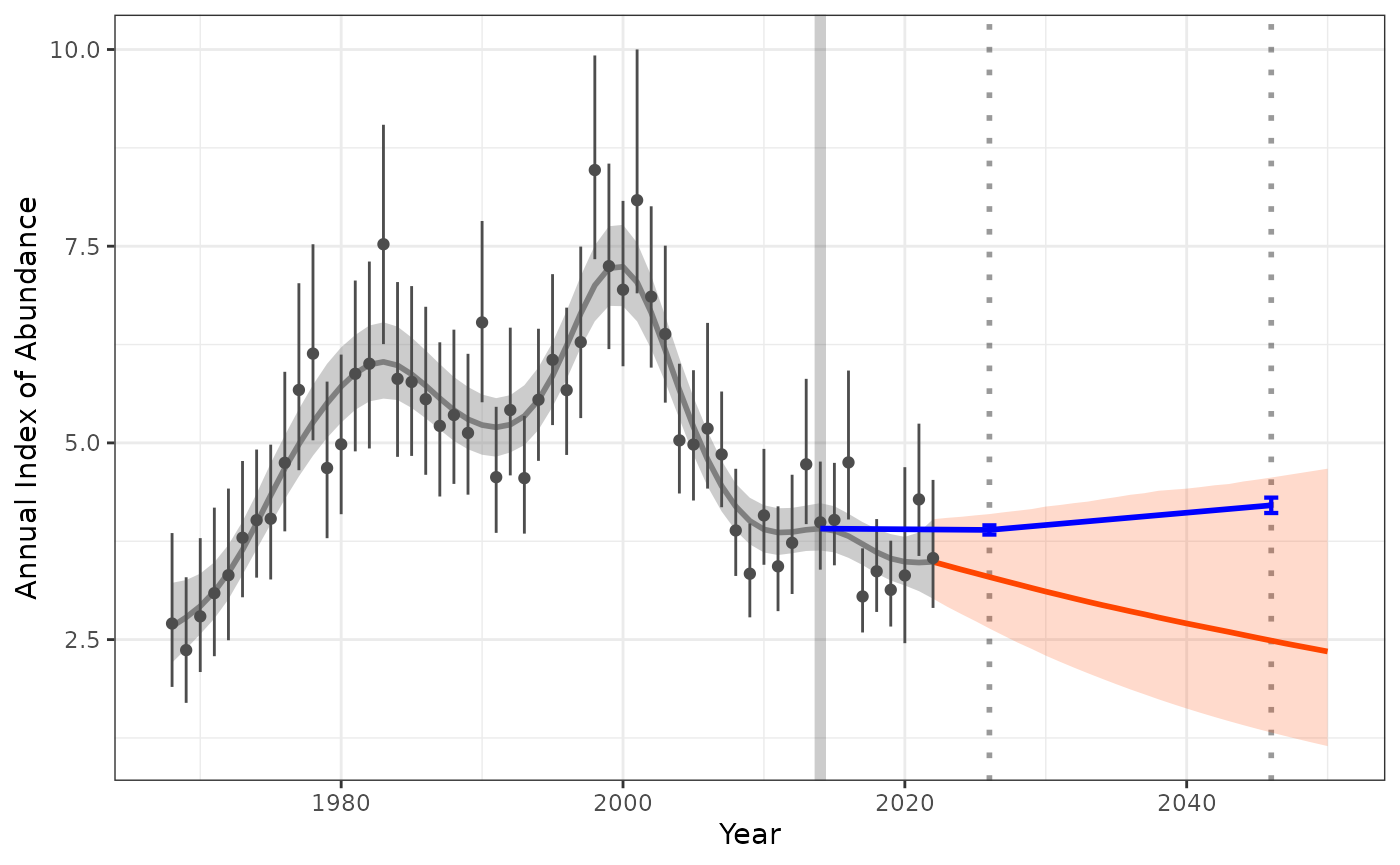

# generate short term plot 
plot_target_previous <- plot_trend(raw_indices = indat1,
                                   model_indices = fitted_data,
                                   pred_indices = proj_trend_previous,
                                   start_yr = 2004,
                                   end_yr = 2014,
                                   ref_yr = 2014,
                                   targets = index_baseline) +
  labs(title = "Projection of trend from 2004-2014") +
  scale_y_continuous(limits = c(0,NA))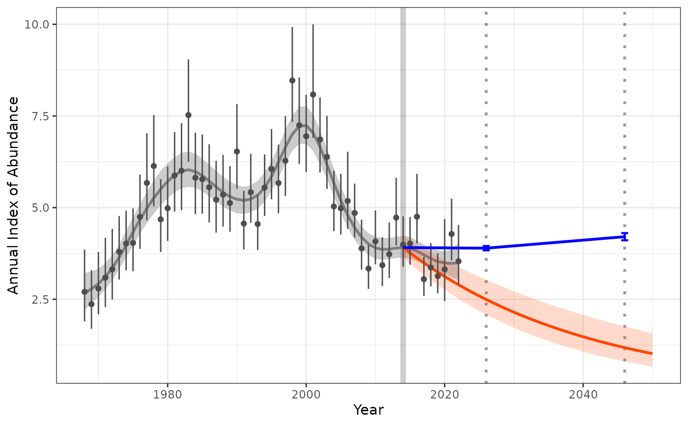

print(plot_target_short / plot_target_previous)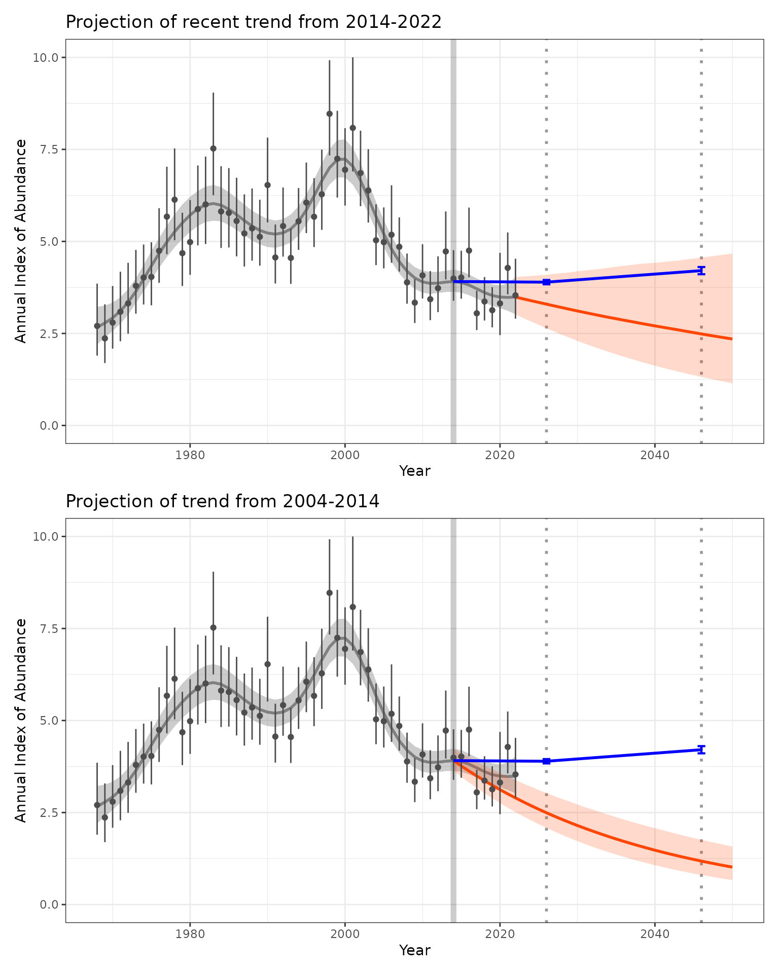

The upper plot shows the projected recent short-term trend, which suggests there is only a small probability of the species meeting the 2026 or 2046 targets (the orange uncertainty bounds only slightly overlaps the blue targets). The lower plot shows that the short-term trend estimated between 2004 and 2014 was more negative than the recent short-term trend.

4. Calculate difference in trends

We can combine the projected estimates for each of the posterior draws and calculate the difference between the two trends.

trend_dif <- trend_previous %>%
  inner_join(trend_short, by = "draw") %>%
  mutate(trend_difference = trend_short-trend_previous)

We can use the difference in probability distributions to quantify the changes between the two trend periods. Lets calculate the 5%, 50% and 95% confidence estimates.

dif_trend <- round(quantile(trend_dif$trend_difference, c(0.05,0.5,0.95)),2)
dif_trend
#>   5%  50%  95% 
#> 0.13 2.27 4.35

The short-term recent trend since 2014 is 2.27% greater from the trend between 2004 and 2014, and that difference is clearly positive, with a 95% confidence interval from 0.13 to 4.35.

This comparison shows that if the short-term trend estimated between 2004 and 2014 had continued, the species would be further from reaching the targets. So while the ongoing decline is troubling, the species recent trends suggest the population is closer to meeting the targets than they were in 2014.

```